
This twin-row planting of honeysuckle protects a 400-foot section of Highway 14 west of Lamberton, MN, in Redwood County. The snow fence is located on the property of the University of Minnesota's Southwest Research and Outreach Center.
Steps used to design a living snow fence given the climatological and topographic characteristics at this site:
- Identify the snowfall over the snow accumulation season (SAS).
- Determine the prevailing winter wind direction by looking at: prevailing wind direction for October–March and the direction of predominant snow transport.
- Determine fetch distance for this site.
- Identify the snow water equivalent (SWE).
- Calculate the mean seasonal snow transport, based on snowfall over the snow accumulation season (SAS).
- Calculate storage capacity, based on fence porosity and height.
- Determine the angle of the prevailing wind with the road.
- Run model to get proper setback distance for fence.
Case Study Results
1. Snowfall

It is necessary to find the mean snowfall in order to calculate the mean seasonal snow transport in a later step.
The snow accumulation season (SAS) is delimited by the dates when average air temperature reaches 0° C, as computed from mean monthly temperatures.
Snowfall over the SAS is the mean monthly snowfall total over the dates of the snow accumulation season.
The 1971-2000 mean snowfall over the SAS is found on the adjacent map. Lamberton is denoted by the star.
The mean snowfall for this case study is 28 inches, or 0.711 meters.
View the SAS section of the mean snowfall page for more information on how this map was made.
2. Wind Direction
Prevailing wind direction and the wind direction of greatest potential snow transport are needed to calculate the attack angle later.
The first table gives the prevailing wind direction for each of the winter months, and the overall prevailing winter wind direction, 310°, or NW. See a degrees vs. cardinal direction table.
| Oct | Nov | Dec | Jan | Feb | Mar | Oct–Mar |
|---|---|---|---|---|---|---|
| 290 | 310 | 310 | 310 | 310 | 310 | 310 |
The second table gives the potential snow transport (Qupot). The direction of greatest snow transport is 310°, or NW.
The prevailing wind direction in this case is therefore 310°, or NW.
| Direction | Qupot (kg/m) |
|---|---|
| 10 | 465 |
| 20 | 58 |
| 30 | 0 |
| 40 | 988 |
| 50 | 3,411 |
| 60 | 5,872 |
| 70 | 3,178 |
| 80 | 872 |
| 90 | 0 |
| 100 | 0 |
| 110 | 116 |
| 120 | 116 |
| 130 | 58 |
| 140 | 58 |
| 150 | 58 |
| 160 | 116 |
| 170 | 291 |
| 180 | 349 |
| 190 | 58 |
| 200 | 116 |
| 210 | 620 |
| 220 | 795 |
| 230 | 349 |
| 240 | 988 |
| 250 | 465 |
| 260 | 814 |
| 270 | 1,299 |
| 280 | 446 |
| 290 | 1,337 |
| 300 | 3,256 |
| 310 | 5,582 |
| 320 | 3,447 |
| 330 | 2,810 |
| 340 | 1,124 |
| 350 | 678 |
| 360 | 620 |
| Total = | 40,813 |
3. Fetch Distance
The fetch distance is used later to calculate mean seasonal snow transport, a variable used to find the ideal snow fence setback.
Fetch can be described as the length of an area that is contributing to blowing snow to a downwind location (Tabler 1994). The upwind boundary may consist of a large ditch, tree line, or farmstead.
For the case study at Lamberton, the fetch distance is 640 meters.

4. Snow Water Equivalent

The snow water equivalent is another piece of data used later to calculate mean seasonal snow transport.
Average snow water equivalent, or the water equivalent of freshly fallen snow, is shown on the map.
For the case study at Lamberton, the snow water equivalent is 0.09. This means that 10 inches of snow is equal to 0.9 inches of liquid precipitation.
View the main snow water equivalent page for more information on how this map was made.
5. Snow Transport

Mean seasonal snow transport is calculated to determine the amount of snow the snow fence will need to contain.
The mean seasonal snow transport (Qt) is calculated using the formula below. The equation utilizes the fetch distance and snow water equivalent found in the previous two steps.
For the case study at Lamberton, the mean season snow transport (Qt) is 16.4 t/m.
Formula for Mean Seasonal Snow Transport
Qt = 1500(S)(SWE)(r)(1-0.14F/3000)
- Qt = mean seasonal snow transport (t/m).
- S = mean snowfall over SAS (m).
- SWE = mean snow water equivalent.
- r = relocation factor for Lamberton, 0.25 (see map).
- F = fetch distance in meters.
6. Snow Storage Capacity
The porosity of the snow fence determines fence's snow storage capacity.
The table below gives the porosity fraction for various snow fences and the resulting snow storage capacity (Qc). Qc is calculated using the formula below.
For the case study at Lamberton, the porosity for the twin-row planting of honeysuckle was 0.70. Assuming the honeysuckle height to be 6.5 feet (1.98 meters), the snow storage capacity was 30.5 t/m.
| Type of Fence | Porosity |
|---|---|
| Solid Fence | 0.0 |
| Double Shrub Row | 0.275 |
| Structural Snow Fence | 0.50 |
| Single Deciduous Tree Row | 0.70 |
| 6-8 Rows Standing Strips of Corn | 0.50 |
Snow Storage Capacity Formula
Qc/H2.2 = (3 + 4P + 44P2 - 60P3)
- Qc is snow storage capacity in t/m.
- H is the fence height in meters.
- P is the porosity percentage of the fence.
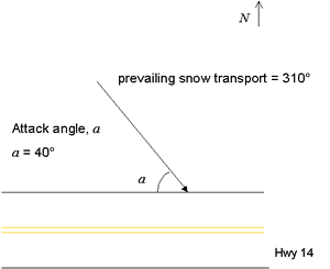
7. Attack Angle
The attack angle of the prevailing winter wind striking the road is used to determine the fence's setback.
The most important consideration for attack angle is the predominant direction of snow transport, or the prevailing direction of the greatest amount of snow transport.
In this case, the wind direction should be taken as 310°.
With an east-west highway, the attack angle of the wind striking the road is 40°.
Wind Variables
| Wind Direction | Degrees |
|---|---|
| Prevailing winter wind direction (Oct-Mar) | 310° |
| Prevailing winter wind direction of snow transport | 310° |
| Wind direction used as attack angle | 310° |
8. Setback
The formula below uses the attack angle, fence height, and porosity to calculate the setback of the fence.
The setback calculated for this case study at Lamberton, MN, is 155 feet (47.1 meters).
Formula for Fence Setback
D = H (sina) (12 + 49P + 7P2 - 37P3)
- D is the setback (m).
- H is the height of the fence (m).
- sina is the attack angle of the prevailing winter wind striking the road.
- P is the porosity percentage of the fence.
Conclusions

The observed snow storage was found to be 16.6 t/m at Lamberton. The storage capacity of this fence design is 30.5 t/m; therefore this design captured roughly 55 percent of capacity for the 2000–01 season.
The calculated setback distance of 155 feet is 5 feet greater than the actual setback of 150 feet. However, no problems occurred at this site because snow deposition did not encroach on the roadway.
References
Gullickson, Dan et al., 1999. Catching the Snow with Living Snow Fences. MnDOT Office of Environmental Services and University of Minnesota Extension Service (MI-7311-S), 140 pp.
Tabler, R.D., 1994. Design Guidelines for the Control of Blowing and Drifting Snow, Strategic Highway Research Program, Washington D.C., 364 pp.